Adapted from Ideals, Varieties, and Algorithms Third Edition, 2007
Appendix C
Computer Algebra Systems
 1 AXIOM
For us, the most important AXIOM commands are [normalForm]?, for doing
the division algorithm, and [groebner]?, for computing a Groebner basis.
A distinctive feature of AXIOM is that every object has a specific type.
In particular, this affects the way AXIOM works with monomial orders:
an order is encoded in a special kind of type. For example, suppose
we want to use lex order on ![\mathbb{Q}[x,y,z] \mathbb{Q}[x,y,z]](images/1339489716636262439-16.0px.png) with
with  .
This is done using the type:
DMP([x,y,z], FRAC INT)
(remember that AXIOM encloses a list inside brackets [...]).
Here DMP stands for "Distributed Multivariate Polynomial", and
FRAC INT means fractions of integers, i.e. rational numbers.
Similarly, grevlex for ![\mathbb{Q}[x,y,z] \mathbb{Q}[x,y,z]](images/1339489716636262439-16.0px.png) with
with  means
using the type:
HDMP([x,y,z],FRAC INT)
where HDMP stands for
"Homogeneous Distributed Multivariate Polynomial". At the end of
the section, we will explain how to get AXIOM to work with grlex
order.
To see how this works in practice, we will divide  by
by
 and
and  using grevlex order with
  . We first
give the three polynomials names and declare their types:
fricas
f : HDMP([x,y], FRAC INT) := x^3+3*y^2
Type: HomogeneousDistributedMultivariatePolynomial
?([x,
y],
Fraction(Integer))
fricas
g : HDMP([x,y], FRAC INT) := x^2+y
Type: HomogeneousDistributedMultivariatePolynomial
?([x,
y],
Fraction(Integer))
fricas
h : HDMP([x,y], FRAC INT) := x+2*x*y
Type: HomogeneousDistributedMultivariatePolynomial
?([x,
y],
Fraction(Integer))
(Here colon : indicates a type declaration. You can save typing
by giving:
HDMP([x,y], FRAC INT)
a symbolic name.) Then the remainder is computed by the command:
fricas
normalForm(f,[g,h])
Type: HomogeneousDistributedMultivariatePolynomial
?([x,
y],
Fraction(Integer))
The output is the remainder of f on division by g, h. In
general the syntax of the command is:
normalForm(poly, polylist)
where poly is the polynomial to be divided by the polynomials in
the list polylist (assuming that everything has been declared to
be of the appropriate type).
To do the same computation using lex order with  , first issue
the command:
fricas
Lex := DMP([x,y], FRAC INT)
Type: Type
to give:
DMP([x,y], FRAC INT)
the symbolic name Lex, and then type:
fricas
normalForm(f::Lex, [g::Lex, h::Lex])
Type: DistributedMultivariatePolynomial
?([x,
y],
Fraction(Integer))
Here, we are using AXIOM's type conversion facility :: to convert
from one type to another.
The syntax for the groebner command is:
groebner(polylist)
This computes a Groebner basis for the ideal generated by the
polynomials in polylist (of the appropriate type). The answer
is reduced in the sense of Chapter 2,  7. For example,
if
 g, h are as above, then the command:
fricas
gb := groebner([g,h])
Type: List(HomogeneousDistributedMultivariatePolynomial
?([x,
y],
Fraction(Integer)))
computes a list (and gives it the symbolic name gb) which is a
Groebner basis for the ideal
![<x^2+y, x+2xy >\ \subset \mathbb{Q}[x,y] <x^2+y, x+2xy >\ \subset \mathbb{Q}[x,y]](images/6999242096768963844-16.0px.png) with respect to grevlex for
with respect to grevlex for  . Also, if you want information
about the intermediate stages of the calculation, you can include
the options "redcrit" or "info" in the
 groebner command. For
example, the command:
fricas
groebner([g,h], "redcrit")

    reduced Critpair - Polynom :

    2   1
   y  + - y
        2

    reduced Critpair - Polynom :

   0

       THE GROEBNER BASIS POLYNOMIALS
Type: List(HomogeneousDistributedMultivariatePolynomial
?([x,
y],
Fraction(Integer)))
will print out the remainders of S-polynomials (only one in this
case) generated during the course of the computation. Adding the
"info" option yields even more information.
AXIOM can also work with coefficients in a variety of fields besides
 . this is easily done by replacing
 FRAC INT in the
type declarations. For instance, to compute Groebner basis over the
field of rational functions in polynomials with integer coefficients,
one uses FRAC POLY INT. To see how this works, let us compute a
Groebner basis for the ideal
![< vx^2+y, uxy+y^2 >\ \subset \mathbb{Q}(u,v)[x,y] < vx^2+y, uxy+y^2 >\ \subset \mathbb{Q}(u,v)[x,y]](images/8162688691955265703-16.0px.png) using lex order with
using lex order with  . This is accomplished by the following
AXIOM commands:
fricas
m : List DMP([x,y], FRAC POLY INT)
Type: Void
fricas
m := [v*x^2 + y, u*x*y + y^2]
Type: List(DistributedMultivariatePolynomial
?([x,
y],
Fraction(Polynomial(Integer))))
fricas
groebner(m)
Type: List(DistributedMultivariatePolynomial
?([x,
y],
Fraction(Polynomial(Integer))))
Notice that this illustrates another method for declaring the type
of polynomials used in a Grobner basis computation.
Other fields are just as easy: one uses FRAC COMPLEX INT for
the field of Gaussian rational numbers
 (note that AXIOM writes
  as
as %i) and PrimeField(p)
for a finite field with p elements (where p is a prime). It
is also possible to compute Groebner bases over arbitrary finite
fields. AXIOM's method of working with finite fields is explained
in Section 8.11 of JENKS and SUTOR (1992) (See:
Axiom Documentation). The ability to "insert" the field you want
to compute Groebner bases over is a good illustration of the power
of AXIOM.
Besides working with lists of polynomials, AXIOM also allows the
user to declare a list of polynomials to be an ideal. The syntax
of the ideal command is:
ideal polylist
where polylist is a list of polynomials of the appropriate type.
This is useful because AXIOM has a number of commands which apply
to ideals (PolynomialIdeals?):
intersect, which computes the intersection of a list of ideals.zeroDim?, which determines (using the methods of Chapter 5,
 3) if the equations have finitely many solutions over an
algebraically closed field.
3) if the equations have finitely many solutions over an
algebraically closed field.dimension, which computes the dimension of the variety
defined by an ideal.prime?, which determines whether an ideal is prime.radical, which computes the radical of an ideal.primaryDecomp, which computes the primary decomposition of
an ideal.
Examples of how to use these and other related commands can be
found in Section 8.12 of JENKS and SUTOR (1992). We should
also mention that there are the commands leadingMonomial and
leadingCoefficient for extracting the leading term and
coefficient of a polynomial.
All of the commands described so far require that you declare
in advance the type of polynomial you'll be using. However, if
you only need Groebner bases in lex or grevlex order with
rational coefficients, then a simpler approach is to use the
AXIOM commands lexGroebner and totalGroebner. For example,
the command:
fricas
lexGroebner([2*x^2+y,2*y^2+x], [x,y])
Type: List(Polynomial(Integer))
computes a Greobner basis (reduced up to constants) for the
ideal
![< 2x^2+y,2y^2+x >\ \subset \mathbb{Q}[x,y] < 2x^2+y,2y^2+x >\ \subset \mathbb{Q}[x,y]](images/2205929710335975140-16.0px.png) using lex order with
using lex order with  . Notice that we didn't have to
declare the type of the polynomials in advance -
 lexGroebner
takes care of this. To do the same computation using grevlex,
simply replace lexGroebner with totalGoebner.
We will end this section by explaining how to get AXIOM to
work with grlex order. All of the raw material need is
present in AXIOM, though it takes a little work to put it
together. For concreteness, suppose we want grlex order on
![\mathbb{Q}[x,y] with \mathbb{Q}[x,y] with](images/5367907374510417903-16.0px.png) x>y$. Then issue the commands:
x>y$. Then issue the commands:
fricas
)set expose add constructor GDMP

   GeneralDistributedMultivariatePolynomial is now explicitly exposed
      in frame initial
fricas
)set expose add constructor ODP

   OrderedDirectProduct is now explicitly exposed in frame initial
Grlex := GDMP([x,y], FRAC INT, ODP(2,NNI,totalLex$ORDFUNS(2,NNI)));
Type: Type
The basic idea here is that GDMP stands for "Generalized
Distributed Multivariate Polynomial", this can be used to
create an AXIOM type for any monomial order, and totalLex
is the function which orders exponent vectors using grlex.
By declaring polynomials to be of type Grlex, you can now
compute Groebner bases using grlex with  .
.
fricas
groebner([g::Grlex, h::Grlex])

   Cannot convert the value from type
      HomogeneousDistributedMultivariatePolynomial([x,y],Fraction(
      Integer)) to GeneralDistributedMultivariatePolynomial([x,y],
      Fraction(Integer),OrderedDirectProduct(2,NonNegativeInteger,
      theMap(ORDFUNS;totalLex;2VB;2,303))) .
We should caution that type conversion doesn't work between
Grlex and the monomial orders created by DMP and HDMP,
though it is possible to write type conversion routines.
fricas
j : Grlex := x^2+y
Type: GeneralDistributedMultivariatePolynomial
?([x,
y],
Fraction(Integer),
OrderedDirectProduct
?(2,
NonNegativeInteger
?,
theMap(ORDFUNS;totalLex;2VB;2,
303)))
fricas
k : Grlex := x+2*x*y
Type: GeneralDistributedMultivariatePolynomial
?([x,
y],
Fraction(Integer),
OrderedDirectProduct
?(2,
NonNegativeInteger
?,
theMap(ORDFUNS;totalLex;2VB;2,
303)))
fricas
groebner([j, k])
Type: List(GeneralDistributedMultivariatePolynomial
?([x,
y],
Fraction(Integer),
OrderedDirectProduct
?(2,
NonNegativeInteger
?,
theMap(ORDFUNS;totalLex;2VB;2,
303))))
Using the AXIOM concept of a package, one could write a
package which knows all of the monomial orders mentioned in
the exercises to Chapter 2,  4, along with commands to
convert one type to the other.
When constructing multivariate polynomials with symbolic parameters variable names (generators)
must be specified. Unspecified names default to parameters. The choice of variables and parameters
will affect the computation of a basis.
fricas
param := FRAC POLY INT
Type: Type
fricas
--vars := [ca,cb,sa,sb,x,y,r1,r2,r3,lab,lac]
--vars := [ca,sa,x,y]
vars := [ca,cb,sa,sb,x,y]
fricas
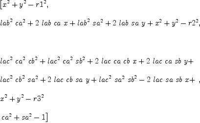
mm:List DMP(vars,param) := [x^2+y^2-r1^2,(x+lab*ca)^2+(y+lab*sa)^2-r2^2,(x+lac*(ca*cb-sa*sb))^2+(y+lac*(sa*cb+ca*sb))^2-r3^2,ca^2+sa^2-1]
Type: List(DistributedMultivariatePolynomial
?([ca,
cb,
sa,
sb,
x,
y],
Fraction(Polynomial(Integer))))
fricas
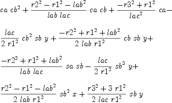
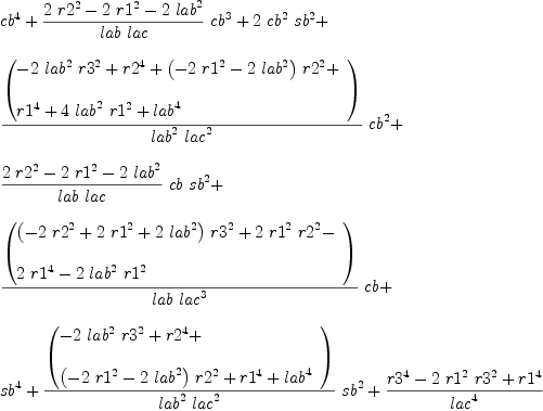
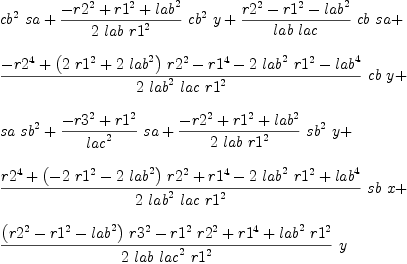
b := groebner(mm); #b
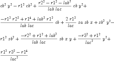
fricas
for i in b repeat
  outputAsTex i
Type: Void
